Spatial Transformer Networks

26 May 2017 | PR12, Paper, Machine Learning, CNN

이번 논문은 Google DeepMind에서 2015년 NIPS에 발표한 “Spatial Transformer Networks”입니다.

이 논문의 저자들은, CNN (Convolutional Neural Network)이 spatially invariant하지 못한 점이 근본적인 한계라고 주장합니다. CNN의 max-pooling layer가 그런 점을 다소 만족시켜 주기는 하지만, $2 \times 2$ 픽셀 단위의 연산으로는 데이터의 다양한 spatial variability에 대처하기 어렵다는 것입니다. 여기서 말하는 spatial variability란 scale (크기 변화), rotation (회전), translation (위치 이동)과 같은 공간적 변화를 의미한다고 보시면 되겠습니다.

이를 해결하기 위해 이 논문에서는 기존 CNN에 끼워 넣을 수 있는 Spatial Transformer라는 새로운 모듈을 제안합니다.

Spatial Transformer의 개념

Spatial transformer란, 기존의 neural network architecture에 집어넣어 아래 그림과 같이 spatial transformation 기능을 동적으로 제공하는 모듈입니다.

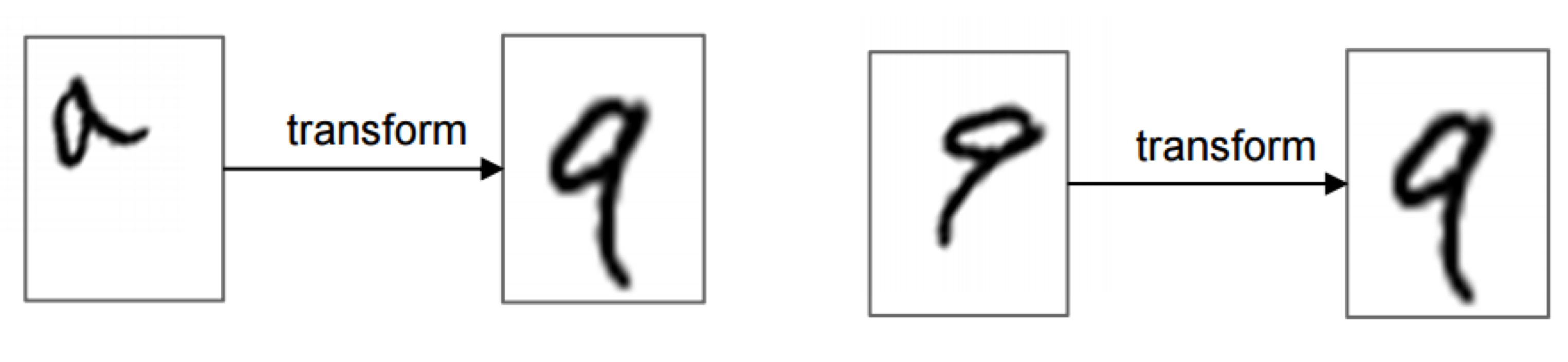
Spatial transformer는 image (또는 feature map)를 입력으로 받아서, scaling, cropping, rotation 뿐만 아니라 thin plate spline과 같은 non-rigid deformation까지 다양하게 지원합니다. 현재 image에서 가장 관련 있는 영역만 골라 선택하거나 (attention), 뒤에 오는 neural network layer의 추론 연산을 돕기 위해 현재의 image (또는 feature map)를 가장 일반적인 (canonical) 형태로 변환하는 등의 용도로 활용할 수 있습니다.

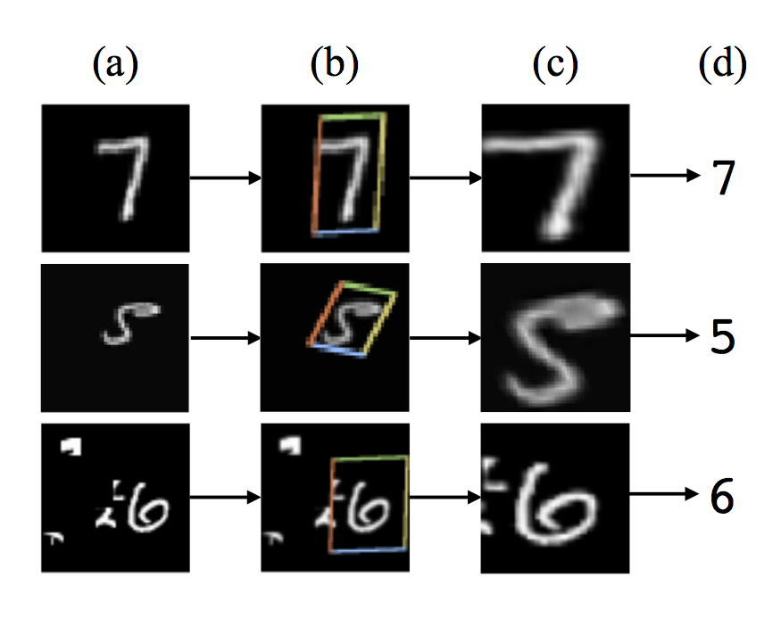
위의 그림은 fully-connected network의 바로 앞 단에 spatial transformer를 사용하고 MNIST digit classification을 위해 training한 결과입니다.

크기와 각도, 중심 위치가 각각인 (a)의 입력들에 대해, spatial transformer는 (b)에 보이는 4각형 영역을 찾아내서 그림 (c)와 같이 변환된 출력을 만들어 fully-connected network에 전달합니다. 그 결과로 classifier가 예측한 숫자 값이 (d)가 됩니다.

Spatial transformer의 동작은 각 입력 데이터 샘플마다 달라지고, 특별한 supervision 없이도 학습 과정에서 습득됩니다. 즉, 사용된 모델의 end-to-end training 과정 중에 backpropagation을 통해 한꺼번에 학습된다는 점이 중요합니다.

Spatial Transformer의 구조

Spatial transformer는 아래 그림과 같이 세 부분으로 구성됩니다.

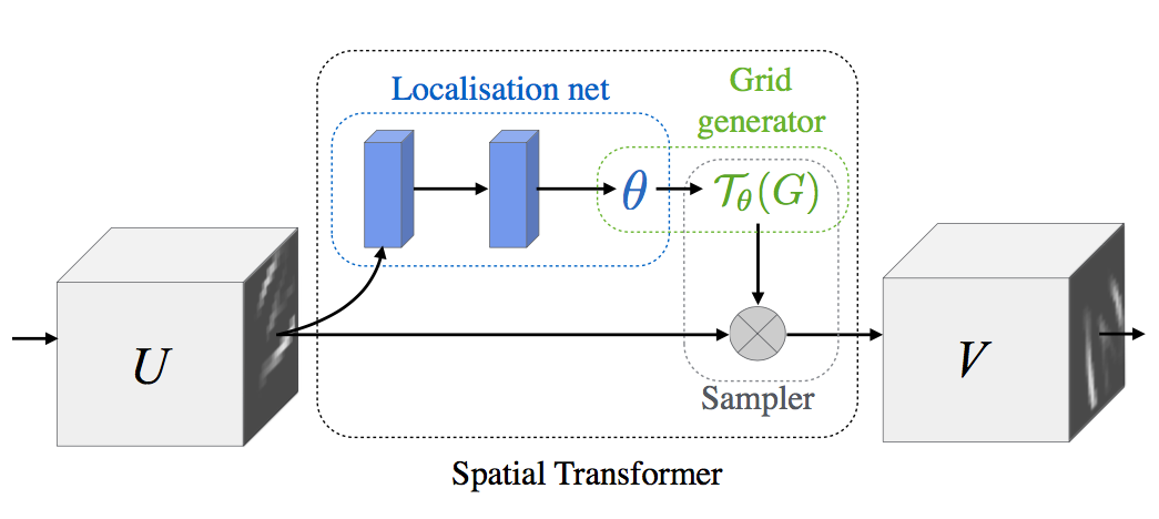
제일 처음, 그 자체로 작은 neural network인 Localisation Network은 input feature map $U$에 적용할 transform의 parameter matrix $\theta$를 추정합니다.

그 다음, Grid Generator는 추정한 $\theta$에 따라 input feature map에서 sampling할 지점의 위치를 정해주는 sampling grid $\mathcal{T}_{\theta}(G)$를 계산합니다.

마지막으로, Sampler는 sampling grid $\mathcal{T}_{\theta}(G)$를 input feature map $U$에 적용해 변환된 output feature map $V$를 만듭니다.

Localisation Network

Localisation network은 input feature map $U$에 적용할 transform의 parameter matrix $\theta$를 추정합니다. 입력 $U \in \mathbb{R}^{H \times W \times C}$은 가로 $W$, 세로 $H$, 채널 수 $C$를 가집니다.

Localisation network은 fully-connected network 또는 convolutional network 모두 가능하며, 마지막 단에 regression layer가 있어 transformation parameter $\theta$를 추정할 수 있기만 하면 됩니다. 이 논문의 실험에서 저자들은 layer 4개의 CNN을 쓰기도 했고 layer 2개의 fully connected network을 사용하기도 했습니다.

Grid Generator

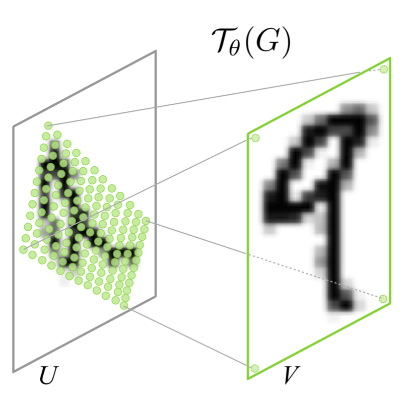
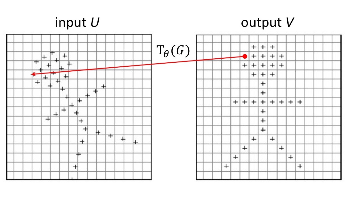
Grid generator는 추정한 $\theta$에 따라 input feature map에서 sampling할 지점의 위치를 정해주는 sampling grid $\mathcal{T}_{\theta}(G)$를 계산합니다.

출력 $V$의 각 pixel $(x_i^t, y_i^t)$은 regular grid (= 일반적인 직사각형 모눈 형태) $G$ 위에 위치하고 있습니다. 출력 $V$의 sampling grid $G$는 transform $\mathcal{T}_{\theta}$ 를 거쳐 입력 $U$의 sampling grid $\mathcal{T}_{\theta}(G)$으로 mapping 됩니다. 이 과정을 그림으로 보이면 아래와 같습니다.

예를 들어 $\mathcal{T}_{\theta}$가 2D affine Transformation $\mathtt{A}_\theta$ 이라면, 아래와 같은 식으로 표현할 수 있습니다.

$$\begin{align} \begin{pmatrix} x_i^s \\ y_i^s \end{pmatrix} = \mathcal{T}_{\theta}(G_i) = \mathtt{A}_\theta \begin{pmatrix} x_i^t \\ y_i^t \\ 1 \end{pmatrix} = \begin{bmatrix} \theta_{11} \,\; \theta_{12} \,\, \theta_{13} \\ \theta_{21} \,\; \theta_{22} \,\; \theta_{23} \end{bmatrix} \begin{pmatrix} x_i^t \\ y_i^t \\ 1 \end{pmatrix} \end{align}$$

Affine transform은 6개의 parameter로 scale, rotation, translation, skew, cropping을 표현할 수 있습니다.

또 한 가지 예로, 3개의 parameter로 isotropic scale (= 가로와 세로 비율이 같은 확대/축소), translation, cropping을 표현하는 attention model은 아래의 수식으로 나타낼 수 있습니다.

$$\begin{align} \begin{pmatrix} x_i^s \\ y_i^s \end{pmatrix} = \mathcal{T}_{\theta}(G_i) = \mathtt{A}_\theta \begin{pmatrix} x_i^t \\ y_i^t \\ 1 \end{pmatrix} = \begin{bmatrix} s \,\; 0 \,\; t_x \\ 0 \,\; s \,\; t_y \end{bmatrix} \begin{pmatrix} x_i^t \\ y_i^t \\ 1 \end{pmatrix} \end{align}$$

Transformation $\mathcal{T}_{\theta}$는 각 parameter에 대해 미분 가능하기만 하면 projective transformation, thin plate spline transformation 등 그 밖의 일반적인 transform을 모두 표현할 수 있습니다.

Sampler

Sampler는 sampling grid $\mathcal{T}_{\theta}(G)$를 input feature map $U$에 적용해 변환된 output feature map $V$를 만듭니다.

출력 $V$에서 특정한 pixel 값을 얻기 위해, 입력 $U$의 어느 위치에서 값을 가져올 지를 sampling grid $\mathcal{T}_{\theta}(G)$가 가지고 있습니다.

(이 그림은 http://northstar-www.dartmouth.edu/doc/idl/html_6.2/Interpolation_Methods.html 에서 가져와 편집했습니다.)

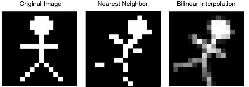
위의 그림에서 보는 것처럼 그 위치가 정확히 정수 좌표 값을 가지지 않을 가능성이 더 높기 때문에, 주변 값들의 interpolation을 통해 값을 계산합니다. 이 과정을 표현하면 아래 식처럼 됩니다.

$$\begin{align} V_i^c = \sum_n^H \sum_m^W U_{nm}^c k(x_i^s - m ; \Phi_x) k(y_i^s - n ; \Phi_y) \quad \forall i \in [1 \ldots H'W'] \, \forall c \in [1 \ldots C] \end{align}$$

Interpolation을 구현하는 함수를 일반적인 sampling kernel $k()$로 표시했기 때문에 어렵게 보입니다만, 그 의미는 어렵지 않습니다. (참고로 Interpolation 이론에 대해서는 Image Processing 과목의 자료에 잘 나와 있습니다. Silvio Savarese의 슬라이드 “Interpolation”를 추천 드립니다

위의 식은 nearest integer interpolation과 bilinear interpolation의 경우 각각 아래와 같은 식이 됩니다.

$$\begin{align} V_i^c = \sum_n^H \sum_m^W U_{nm}^c \delta(\lfloor x_i^s + 0.5 \rfloor - m) \delta(\lfloor y_i^s + 0.5 \rfloor - n) \end{align}$$ $$\begin{align} V_i^c = \sum_n^H \sum_m^W U_{nm}^c \max(0, 1-\lvert x_i^s - m\rvert) \max(0, 1-\lvert y_i^s - n\rvert) \end{align}$$

이 두 가지 interpolation을 적용한 간단한 예를 아래 그림에 보입니다.

전체 네트워크에서 loss 값을 backpropagation으로 계산하려면 $U$와 $G$에 대해 미분 가능해야 합니다. Bilinear interpolation의 경우 각각의 partial derivative를 구해보면 아래 식과 같습니다.

$$\begin{align} \frac{\partial V_i^c}{\partial U_{nm}^c} = \sum_n^H \sum_m^W \max(0, 1-\lvert x_i^s - m\rvert) \max(0, 1-\lvert y_i^s - n\rvert) \end{align}$$ $$\begin{align} \frac{\partial V_i^c}{\partial x_{i}^s} = \sum_n^H \sum_m^W U_{nm}^c \max(0, 1-\lvert y_i^s - n\rvert) \begin{cases} 0 \quad \text{if} \; \lvert m - x_i^s \rvert \ge 1 \\ 1 \quad \text{if} \; m \ge x_i^s \\ -1 \quad \text{if} \; m \lt x_i^s \end{cases} \end{align}$$

$\frac{\partial V_i^c}{\partial y_{i}^s}$의 식도 마찬가지로 구할 수 있습니다. Sampling function이 모든 구간에서 미분가능하지 않은 경우에도, 구간별로 나눠 subgradient를 통해 backpropagation을 계산할 수 있습니다.

Spatial Transformer Networks

Localisation network, grid generator와 sampler로 구성한 spatial transformer module을 CNN 구조에 끼워 넣은 것을 Spatial Transformer Network이라고 합니다. Spatial transformer module은 CNN의 어느 지점에나, 몇 개라도 이론상 집어넣을 수 있습니다.

Spatial transformer가 어떻게 input feature map을 transform할 지는 CNN의 전체 cost function을 최소화하는 training 과정 중에 학습됩니다. 따라서 전체 training 속도에 미치는 영향이 거의 없다고 저자들은 주장합니다.

Spatial transformer module을 CNN의 입력 바로 앞에 배치하는 것이 가장 일반적이지만, network 내부의 깊은 layer에 배치해 좀더 추상화된 정보에 적용을 한다거나 여러 개를 병렬로 배치해서 한 image에 속한 여러 부분을 각각 tracking하는 용도로 사용할 수도 있다고 합니다. 복수의 spatial transformer module을 동시에 적용하는 실험 결과가 뒷 부분에 있는 동영상에서 MNIST Addition이라는 이름으로 소개됩니다.

실험 결과

Supervised learning 문제에 대해 spatial transformer network를 적용하는 몇 가지 실험 결과를 보겠습니다.

Distorted MNIST

먼저, distorted된 MNIST 데이터셋에 대해 spatial transformer로 classification 성능을 개선하는 실험입니다.

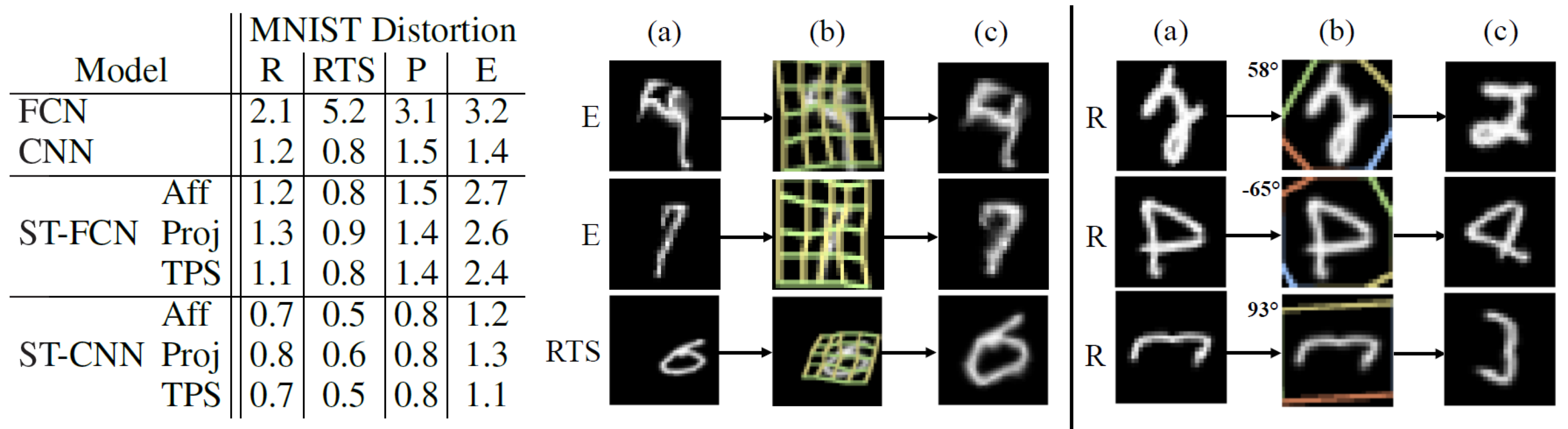
이 실험에서 사용된 MNIST 데이터는 4가지 방법으로 distorted 되었습니다: rotation (R), rotation-translation-scale (RTS), projective transformation (P), elastic warping (E)

모델로는 기본 FCN과 CNN, 그리고 각각 앞 단에 spatial transformer를 추가한 ST-FCN과 ST-CNN을 사용했습니다. CNN에는 2개의 max-pooling layer가 있습니다.

아래의 실험 결과에서 ST-CNN이 가장 성능이 좋은 것을 알 수 있습니다. CNN이 FCN 보다 더 성능이 좋은 것은 max-pooling layer가 spatial invariance에 기여하고 convolutional layer가 모델링을 더 잘하기 때문일 것으로 보입니다.

한편, 같은 모델 안에서는 TPS transformation이 가장 좋은 성능을 보였습니다.

아래 YouTube 비디오는 이 논문의 저자가 직접 공개한 실험 결과를 요약한 동영상입니다. 이 논문에서 상세히 다루지 않은 MNIST addition 실험(2개의 숫자 동시 인식)과 co-localisation (수십 개의 숫자 인식) 실험도 추가되어 있습니다.

Stree View House Numbers

두 번째로, 20만 개의 실제 집 주소 표지의 사진으로 구성된 Street View House Numbers (SVHN) 데이터셋에서 숫자를 인식하는 실험입니다.

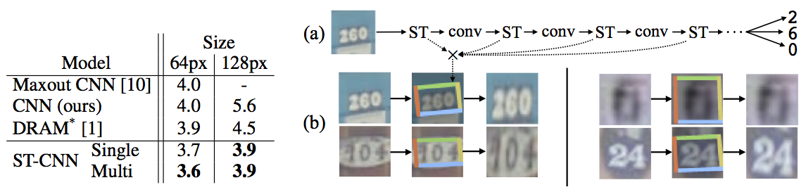
이 실험에서는 아래 그림의 (a)와 같이 CNN의 convolutional stack 부분에 복수의 spatial transformer를 삽입해서 사용했습니다.

모델로는 기본 CNN 모델 (11개 hidden layer)과 ST-CNN Single, ST-CNN Multi를 사용했습니다. ST-CNN Single은 CNN 입력 단에 4-layer CNN으로 구성된 spatial transformer를 추가한 것입니다. ST-CNN Multi은 아래 그림의 (a)와 같이 CNN의 처음 4개의 convolutional layer 앞 단에 2-layer FCN spatial transformer를 하나씩 삽입한 모델입니다. 즉 뒤 3개의 spatial transformer는 convolutional feature map을 transform하는 용도입니다. 모든 spatial transformer에는 affine transformation과 bilinear sampler를 사용했습니다.

실험 결과, ST-CNN Multi 모델이 가장 높은 성능을 보였는데 그럼에도 기본 CNN 모델보다 6%만 느려졌다고 합니다.

Fine-Grained Classification

세 번째로, 200종의 새 사진 11,788장으로 구성된 Caltech의 CUB-200-2011 birds 데이터셋에 fine-grained bird classification을 적용한 실험입니다.

기본 모델은 Inception architecture에 batch normalisation을 사용한 강력한 CNN 구조(Sergey Ioffe의 논문 “Batch Normalization: Accelerating Deep Network Training by Reducing Internal Covariate Shift”)입니다.

이 모델에 추가로 spatial transformer 2개($2 \times$ST-CNN) 또는 4개($4 \times$ST-CNN)를 병렬로 사용해서 자동으로 object에서 중요한 부분을 attention하게 학습했습니다.

실험 결과, 모든 ST-CNN이 기존 CNN보다 높은 성능을 보였습니다. 아래 그림에서 위 줄의 그림은 $2 \times$ST-CNN의 결과이고 아래 줄의 그림은 $2 \times$ST-CNN의 결과입니다.

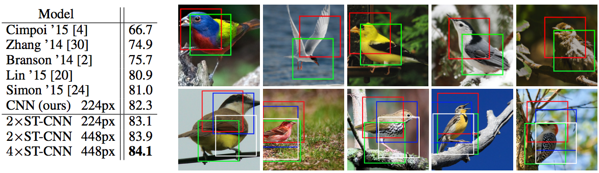
여기서 주목할 점은 red 박스는 새의 head 부분을, green 박스는 body의 중심 부분을 찾도록 별도의 supervision 없이 스스로 학습되었다는 것입니다.

비교: Deformable Convolutional Networks

마지막으로, 앞에서 다른 post에 소개했던 2017년의 “Deformable Convolutional Networks” 연구와 비교해 보겠습니다.

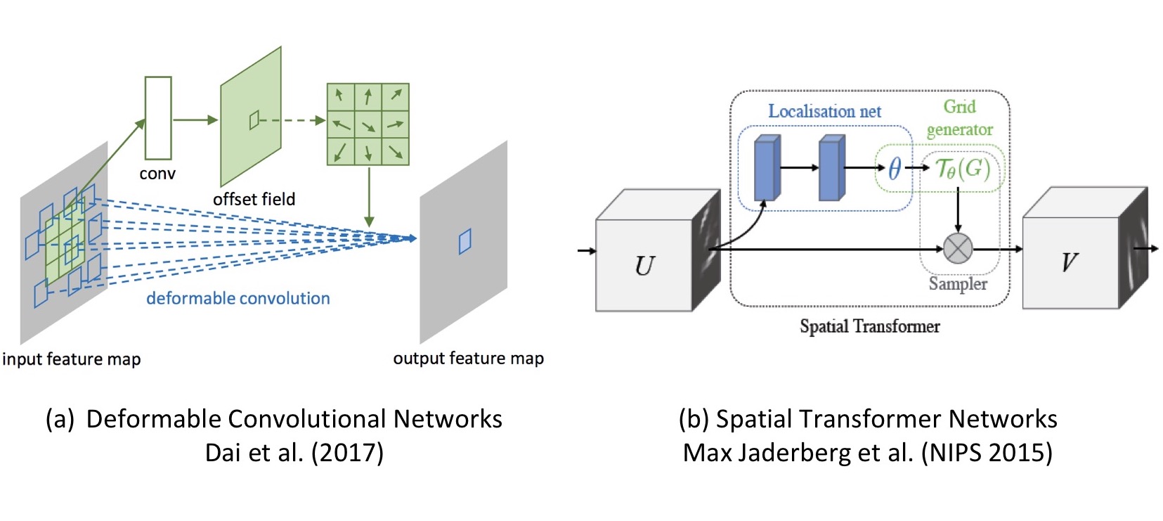
이 두 논문은 공통적으로 내부의 transformation parameter를 데이터로부터 학습한다는 특징이 있습니다.

차이점으로는, spatial transformer networks는 parameter로 transform matrix (affine의 경우 6개 element)면 충분한 반면, deformable convolution networks는 sampling grid의 모든 pixel에 대해 offset 값이 필요합니다.

또한, spatial transformer networks는 input $U$에서 output $V$로 mapping하는 연산이 explicit하게 필요하지만, deformable convolution networks는 그 과정이 원래의 convolution 연산에 포함되어 별도로 필요하지 않습니다.

그밖에, deformable convolution networks 논문의 저자들은 spatial transformer networks가 thin plate spline과 같은 warping을 지원할 수 있지만 그만큼 연산이 많이 필요하다고 주장하고 있습니다.

– Jamie;

References

• Max Jaderberg의 논문 “Spatial Transformer Networks”
• Max Jaderberg의 발표 동영상 “Symposium: Deep Learning - Max Jaderberg”
• GitHub의 Lasagne의 example
• Tensorflow GitHub의 Spatial Transformer Networks
• Xavier Giro의 슬라이드 “Spatial Transformer Networks”
• Okay Arik의 슬라이드 “Spatial Transformer Networks”
• Kevin Nguyen의 Medium article “Spatial Transformer Networks with Tensorflow”
• Kevin Nguyen의 GitHub “Spatial Transformer Example with Cluttered MNIST”
• Alban Desmaison의 torch article “The power of Spatial Transformer Networks”
• Kevin Zakka의 blog post “Deep Learning Paper Implementations: Spatial Transformer Networks - Part I”
• Silvio Levy의 Affine Transformations
• Wikipedia의 Bilinear interpolation
• Silvio Levy의 Projective Transformations
• Wikipedia의 Thin plate spline
• Wikipedia의 Subgradient method
• Aaron Anderson의 Subgradient optimization
• Silvio Savarese의 슬라이드 “Interpolation”
• Yann LeCun의 MNIST dataset
• Stanford의 Street View House Numbers (SVHN) dataset
• Caltech의 CUB-200-2011 birds dataset
• Stanford의 ImageNet dataset
• Sergey Ioffe의 논문 “Batch Normalization: Accelerating Deep Network Training by Reducing Internal Covariate Shift”
• Jifeng Dai의 논문 “Deformable Convolutional Networks”